Python Extended API

We aimed to structure our code in the most general way to derive at our analysis. We want to share our structure to potentially help everyone to improve their code organization.

Hence, we share here how we use the classes defined in polarityJaM as a library.

You can find this notebook here!

%load_ext autoreload
%autoreload 2

# must run in an environment where polarityJaM is installed
from polarityjam import Extractor, Plotter, PropertiesCollection
from polarityjam import RuntimeParameter, PlotParameter, SegmentationParameter, ImageParameter
from polarityjam import BioMedicalMask, BioMedicalInstanceSegmentationMask
from polarityjam import BioMedicalImage
from polarityjam import BioMedicalInstanceSegmentation
from polarityjam import load_segmenter
from polarityjam.utils.io import read_image
from pathlib import Path

Setup data

First, lets setup the data we want to use. You find the images in our example dataset that are part of polarityJaM. Here is the link to the example data! Simply extract the zip and have it in the same directory as this file.

### ADAPT ME ###
path_root = Path("")
input_file1 = path_root.joinpath("data/golgi_nuclei/set_2/060721_EGM2_18dyn_02.tif")
input_file2 = path_root.joinpath("data/golgi_nuclei/set_1/060721_EGM2_18dyn_01.tif")

output_path = path_root.joinpath("polarityjam_out/")
output_file_prefix1 = "060721_EGM2_18dyn_02"
output_file_prefix2 = "060721_EGM2_18dyn_01"
### ADAPT ME ###

Now, we define the parameters of the image. This depends on your question you are trying to answer and your experimental setup.

# read input
img1 = read_image(input_file1)
img2 = read_image(input_file2)

# parameters
params_image1 = ImageParameter()

params_runtime = RuntimeParameter()
params_seg = SegmentationParameter(params_runtime.segmentation_algorithm)
params_plot = PlotParameter()

# set the image parameters
params_image1.channel_organelle = 0  # golgi channel
params_image1.channel_nucleus = 2
params_image1.channel_junction = 3
params_image1.channel_expression_marker = 3
params_image1.pixel_to_micron_ratio = 2.4089  # from the biological setup

# same experimental setup
params_image2 = params_image1

print(params_image1)

ImageParameter:
channel_junction              3
channel_nucleus               2
channel_organelle             0
channel_expression_marker     3
pixel_to_micron_ratio         2.4089

Segmentation & Feature Extraction

Here, we prepare the segmentation of the images. Here, cellpose is used to segment the image.

# Define your segmenter and segment your image
cellpose_segmentation, params_seg = load_segmenter(params_runtime)  # take default segmentation parameters for the chosen algorithm
# alternatively, you can pass your own parameters as a dictionary or SegmentationParameter object
# cellpose_segmentation, params_seg = load_segmenter(params_runtime, params_seg)
# cellpose_segmentation, params_seg = load_segmenter(params_runtime, {"cellprob_threshold": 0.5})
img_channels, _ = cellpose_segmentation.prepare(img1, params_image1)
mask1 = cellpose_segmentation.segment(img_channels, input_file1)

img_channels, _ = cellpose_segmentation.prepare(img2, params_image2)
mask2 = cellpose_segmentation.segment(img_channels, input_file2);

cellprob_threshold and dist_threshold are being deprecated in a future release, use mask_threshold instead

Now we can extract the features of both images. We collect them in a single collection object that is automatically saved in the outputpath.

# feature extraction
collection = PropertiesCollection()
extractor = Extractor(params_runtime)
extractor.extract(img1, params_image1, mask1, output_file_prefix1, output_path, collection)
extractor.extract(img2, params_image2, mask2, output_file_prefix2, output_path, collection);  # gather features in the same collection

Working with the pyplot visualization

Not being able to alter plots can be dissatisfying. Hence, we return the figure and their axes to let you modify basic things that are specific to your setup. Like a title for example

# plot the cell orientation of a specific image in your collection
plotter = Plotter(params_plot)

# plot the cell orientation of a specific image in your collection
f, ax = plotter.plot_shape_orientation(collection, "060721_EGM2_18dyn_02", params_runtime.cue_direction)  # image is automatically saved in output_path

# alter the plot to your desires; caution: changes will not be automatically saved!
ax[0].set_title("Cell orientation experiment condition 1")
ax[1].set_title("Nucleus orientation experiment condition 1");

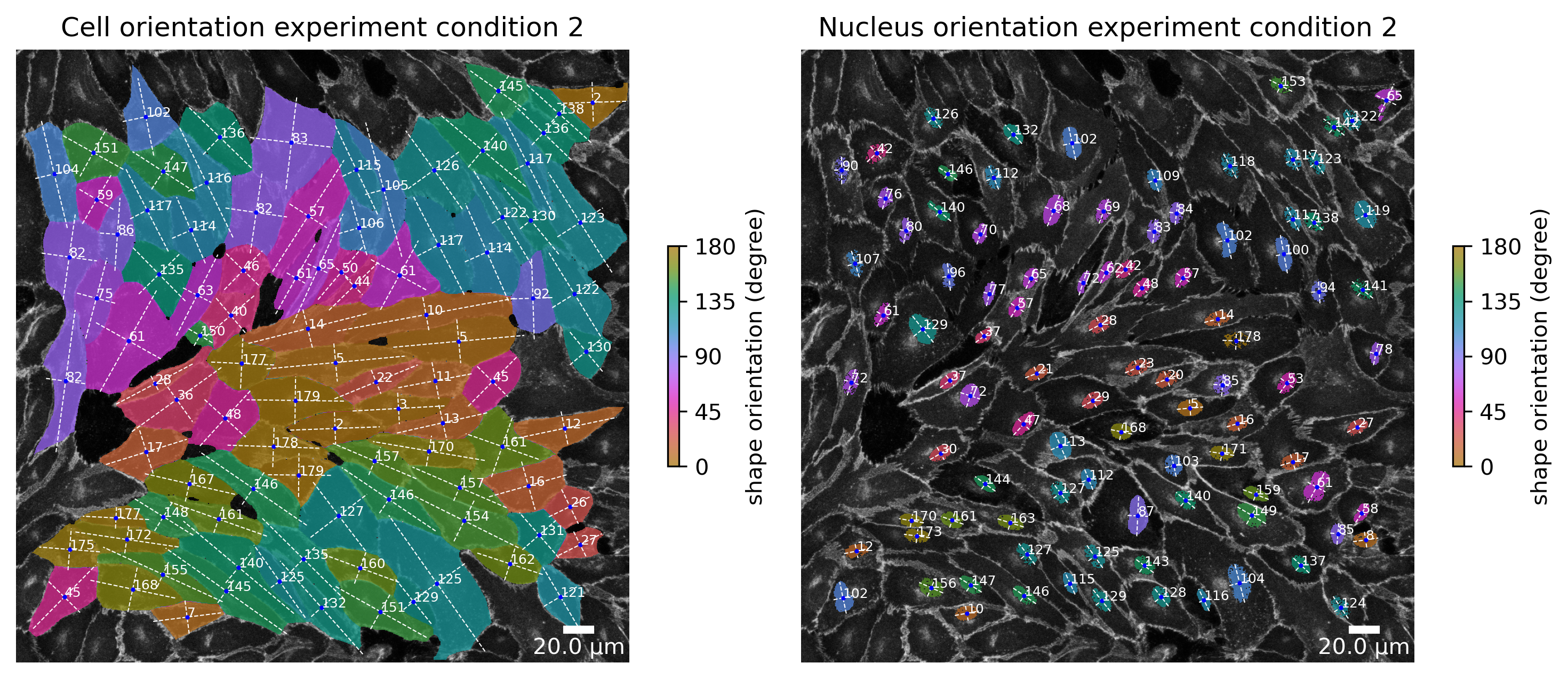
f, ax = plotter.plot_shape_orientation(collection, "060721_EGM2_18dyn_01", params_runtime.cue_direction)  # image is automatically saved in output_path
ax[0].set_title("Cell orientation experiment condition 2")
ax[1].set_title("Nucleus orientation experiment condition 2");

Working with a BioMedicalImage, Channels and simple Masks

Dealing with masks and channels can be confusing. We provide masks classes for you that facilitates basic operations. Here you see examples of how to perform some basic operations without using sometimes confusing numpy operations. Don’t worry, you can always perform any operation with numpy by accessing the <object>.data numpy array attribute of your object and turn it back to a segmentation mask afterwards.

from polarityjam.vizualization.plot import add_scalebar, add_colorbar
from matplotlib import pyplot as plt
import cmocean as cm

# turn your image to a BioMedicalImage to get access to enhanced functionality
bio_med_image = BioMedicalImage(img1, params_image1)

# get a simple segmentation from the channel by otsu thresholding
nuc_mask = BioMedicalMask.from_threshold_otsu(bio_med_image.nucleus.data)
nuc_mask_invert = nuc_mask.invert()

masked_junction_channel = bio_med_image.junction.mask(nuc_mask_invert)

# look at our results
fig, axes = plt.subplots(1, 4, figsize=(params_plot.graphics_width, params_plot.graphics_height))
cax0 = axes[0].imshow(bio_med_image.junction.data, cmap=cm.cm.gray)
cax1 = axes[1].imshow(bio_med_image.nucleus.data, cmap=cm.cm.gray)
cax3 = axes[2].imshow(nuc_mask.data, cmap=cm.cm.gray)
cax2 = axes[3].imshow(masked_junction_channel.data, cmap=cm.cm.gray)

# enhance plots
axes[0].set_title("Junction channel", fontsize=3)
axes[1].set_title("Nucleus channel", fontsize=3)
axes[2].set_title("Nucleus semantic segmentation mask", fontsize=3)
axes[3].set_title("Nucleus masked junction channel", fontsize=3)
[ax.axis('off') for ax in axes];

Working with instance and semantic masks

Sometimes, it is of advantage to look at a single cell isolated from the others. Here, you can see how you would achieve this using the PolarityJaM library and its mask classes

# options
instance_label = 70
outline_width = 10

# turn your segmentation mask to a BioMedicalMask to get access to enhanced functionality
bio_med_segmentation_mask = BioMedicalInstanceSegmentationMask(mask1)

# get a single instance
single_instance_mask = bio_med_segmentation_mask.get_single_instance_mask(instance_label)  # mask is now a semantic mask!

# get the outline of the cell of a certain width
single_instance_outline_mask = single_instance_mask.get_outline_from_mask(outline_width)

# apply masks on a channel from our image
junction_channel_masked = bio_med_image.junction.mask(single_instance_mask)
junction_channel_masked_outline = bio_med_image.junction.mask(single_instance_outline_mask)

# visualize junction channel with our single instance mask
fig, axes = plt.subplots(1, 2, figsize=(params_plot.graphics_width, params_plot.graphics_height))
cax1 = axes[0].imshow(junction_channel_masked.data, cmap=cm.cm.gray)
cax2 = axes[1].imshow(junction_channel_masked_outline.data, cmap=cm.cm.gray)

# enhance plot
axes[0].set_title("Cell instance 70")
axes[1].set_title("Cell instance 70 - outline")
[ax.axis('off') for ax in axes];

Working with the extracted features

Main focus is the feature extraction process of PolarityJaM. Here we show how you can access features in your collection and use them to do an enhanced visualization.

# get a specific image feature from the collection as a pandas dataset. A list of all available properties are listed here:
# https://polarityjam.readthedocs.io/en/latest/Features.html
cell_orientation_img1 = collection.get_properties_by_img_name("060721_EGM2_18dyn_02")["cell_shape_orientation_deg"]

# alter the features to our desires by applying a filter
cell_orientation_img1_masked = cell_orientation_img1.where(
    cell_orientation_img1 > 45, bio_med_segmentation_mask.background_label
).where(
    cell_orientation_img1 < 135, bio_med_segmentation_mask.background_label
)
# prepare our segmentation mask. We used clear border and remove small objects during feature extraction
bio_med_segmentation_mask_c_r = bio_med_segmentation_mask.clear_border().remove_small_objects(10)

# apply this new feature vector to the instance segmentation mask.
# Please note that order matters! We could however, pass a mapping to the relabel function (not shown here).
bio_med_segmentation_mask_relabeled = bio_med_segmentation_mask_c_r.relabel(cell_orientation_img1_masked.values)

# visualize
fig, ax = plt.subplots(1, 1, figsize=(params_plot.graphics_width, params_plot.graphics_height))
cax1 = ax.imshow(bio_med_image.junction.data, cmap=cm.cm.gray)  # use ".data" to get to your numpy channel image
cax2 = ax.imshow(bio_med_segmentation_mask_relabeled.mask_background().data, cmap=cm.cm.phase, alpha=0.75)
add_scalebar(
    ax,
    params_plot.length_scalebar_microns,
    params_image1.pixel_to_micron_ratio,
    int(params_plot.length_scalebar_microns / 2),
    "w"
)
add_colorbar(
    fig, cax2, ax, [45.0, 90.0, 135.0], "circularity"
)
ax.set_title("Cell shape orientation between 45 and 135 degrees")
ax.axis('off');

Working with the feature objects

Lets look at the feature objects that are available in PolarityJaM. First, we will use the two segmentation masks we created earlier and use them to create an instance segmentation object. This object can be attached to our image to get access to the features that are based on the instance segmentation.

organelle_mask = BioMedicalMask.from_threshold_otsu(bio_med_image.organelle.data)

# create an instance segmentation object
segmentation = BioMedicalInstanceSegmentation(
    bio_med_segmentation_mask,
    connection_graph=True,
    segmentation_mask_nuclei=nuc_mask.overlay_instance_segmentation(bio_med_segmentation_mask),  # make sure we have a nuclei instance segmentation mask with the same labels
    segmentation_mask_organelle=organelle_mask.overlay_instance_segmentation(bio_med_segmentation_mask)
)
# attach the segmentation to our image
bio_med_image.segmentation = segmentation

# use the image to get access to the features
focused_image = bio_med_image.focus(70, outline_width)

# access the junction features
junction_properties = focused_image.get_junction_properties(params_runtime)

print(junction_properties.straight_line_junction_length)
print(junction_properties.junction_cue_directional_intensity_ratio)
print(junction_properties.junction_cue_axial_intensity_ratio)

345.23352921351915
0.03228602949373771
0.5032425678760815

organelle_mask = BioMedicalMask.from_threshold_otsu(bio_med_image.organelle.data)

# create an instance segmentation object
segmentation = BioMedicalInstanceSegmentation(
    bio_med_segmentation_mask,
    connection_graph=True,
    segmentation_mask_nuclei=nuc_mask.overlay_instance_segmentation(bio_med_segmentation_mask),  # make sure we have a nuclei instance segmentation mask with the same labels
    segmentation_mask_organelle=organelle_mask.overlay_instance_segmentation(bio_med_segmentation_mask)
)
# attach the segmentation to our image
bio_med_image.segmentation = segmentation

# use the image to get access to the features
focused_image = bio_med_image.focus(70, outline_width)

# access the junction features
junction_properties = focused_image.get_junction_properties(params_runtime)

print(junction_properties.straight_line_junction_length)
print(junction_properties.junction_cue_directional_intensity_ratio)
print(junction_properties.junction_cue_axial_intensity_ratio)

345.23352921351915
0.03228602949373771
0.5032425678760815