OMERO and Polarity-JaM
OMERO is a client-server software for visualizing, managing, and annotating microscope images. It is used by many research institutions to store and manage their microscopy data. PolarityJaM can be used to analyze images stored in OMERO. This notebook demonstrates how to connect to an OMERO server, load an image, and analyze it with Polarity-JaM.
Installation
To use PolarityJaM with OMERO, you need to install the OMERO Python client. You can install it with pip in your environment where Polarity-JaM is installed:
micromamba activate polarityjam
pip install omero-py
Connection to OMERO
You can use PolarityJaM with OMERO in the same way as with local images. You need to load the image from OMERO, convert it to a numpy array, and then analyze it with PolarityJaM.
You might need to adjust the connection parameters to your OMERO server.
[ ]:
### ADAPT ME ###
HOSTNAME = "myomero.my-domain.net"
PORT = int(4064)
### ADAPT ME ###
[ ]:
from omero.gateway import BlitzGateway
from getpass import getpass

# connect to omero
conn = BlitzGateway(
    input("Username: "), getpass("Password: "), host=HOSTNAME, port=PORT, secure=True
)
conn.connect()
User and Group Information
Sometimes you need to know which groups the user is a member of or switch the group to access the images. You can get this information with the following commands.
[ ]:
print("Groups the user is a member of:")
for g in conn.getGroupsMemberOf():
    print("Group: %s \tID: %s" % (g.getName(), g.getId()))
print(f"Current group: {conn.getGroupFromContext().getName()}")

# switch group
conn.setGroupForSession(203)
print(f"Current group: {conn.getGroupFromContext().getName()}")
Load Image from Omero
You can load an image from OMERO with the image ID. You can find the image ID in the OMERO web interface. Here we load our example image.
[24]:
img_060721_EGM2_18dyn_02_omero_id = 30618

img_omero = conn.getObject("Image", img_060721_EGM2_18dyn_02_omero_id)
[25]:
assert img_omero is not None, "Image not found"
Lets check the image shape and convert it to a numpy array.
[26]:
img_omero
[26]:

|
Image information
|
|
[27]:
import numpy as np
from pathlib import Path

# get image shape
shape = img_omero.getSizeZ(), img_omero.getSizeT(), img_omero.getSizeC(), img_omero.getSizeX(), img_omero.getSizeY()
print("Image shape: ZTCXY", shape)

# convert to numpy array
pxls = img_omero.getPrimaryPixels()
img = np.zeros([img_omero.getSizeX(), img_omero.getSizeY(), img_omero.getSizeC()])
for i in range(img_omero.getSizeC()):
    img[:, :, i] = pxls.getPlane(0, i, 0)

print("Numpy Image shape: ", img.shape)
Image shape: ZTCXY (1, 1, 4, 1024, 1024)
Numpy Image shape:  (1024, 1024, 4)
[ ]:
### ADAPT ME ###
path_root = Path("")
output_path = path_root.joinpath("polarityjam_out")
### ADAPT ME ###
[ ]:
input_file = img_omero.getName()
output_file_prefix = Path(input_file).stem

print("Input file: ", input_file)
print("Output path: ", output_path)
print("Output file prefix: ", output_file_prefix)
Analysis
Lets analyze the image with PolarityJaM. We first need to define the parameters for the image, runtime, and plotting. Then we can segment the image and extract features to finally plot the results.
Note
This part is similar to the local analysis. See the notebook PolarityJaM for more details.
[29]:
# must run in an environment where polarityJaM and omero-py is installed
from polarityjam import Extractor, Plotter, PropertiesCollection
from polarityjam import RuntimeParameter, PlotParameter, ImageParameter
from polarityjam import PolarityJamLogger
from polarityjam import load_segmenter

plog = PolarityJamLogger("WARNING")

# describe your image with ImageParameter
params_image = ImageParameter()

# set the channels
params_image.channel_organelle = 0  # golgi channel
params_image.channel_nucleus = 2
params_image.channel_junction = 3
params_image.channel_expression_marker = 3
params_image.pixel_to_micron_ratio = 2.4089

# define other parameters, use default values
params_runtime = RuntimeParameter()
params_plot = PlotParameter()

# change some parameters
params_runtime.membrane_thickness = 6
params_runtime.min_organelle_size = 9

print(params_image)
print(params_runtime)
print(params_plot)
ImageParameter:
channel_junction              3
channel_nucleus               2
channel_organelle             0
channel_expression_marker     3
pixel_to_micron_ratio         2.4089

RuntimeParameter:
extract_group_features        False
membrane_thickness            6
junction_threshold            -1
feature_of_interest           cell_area
min_cell_size                 50
min_nucleus_size              10
min_organelle_size            9
dp_epsilon                    5
cue_direction                 0
connection_graph              True
segmentation_algorithm        CellposeSegmenter
remove_small_objects_size     10
clear_border                  True
save_sc_image                 False
keyfile_condition_cols        ['short_name']

PlotParameter:
plot_junctions                True
plot_polarity                 True
plot_elongation               True
plot_circularity              True
plot_marker                   True
plot_ratio_method             True
plot_shape_orientation        True
plot_foi                      True
plot_sc_image                 False
plot_threshold_masks          None
plot_sc_partitions            False
show_statistics               False
show_polarity_angles          True
show_graphics_axis            False
show_scalebar                 True
outline_width                 2
length_scalebar_microns       20.0
graphics_output_format        ['png']
dpi                           300
graphics_width                5
graphics_height               5
membrane_thickness            5
fontsize_text_annotations     6
font_color                    w
marker_size                   2
alpha                         0.7
alpha_cell_outline            1.0
[30]:
print("Used algorithm for segmentation: %s " % params_runtime.segmentation_algorithm)
Used algorithm for segmentation: CellposeSegmenter
[14]:
# Now define your segmenter and segment your image with the default algorithm and default parameters.
cellpose_segmentation, _ = load_segmenter(params_runtime)
# prepare your image for segmentation
img_prepared, img_prepared_params = cellpose_segmentation.prepare(img, params_image)
# now segment your prepared image to get the masks
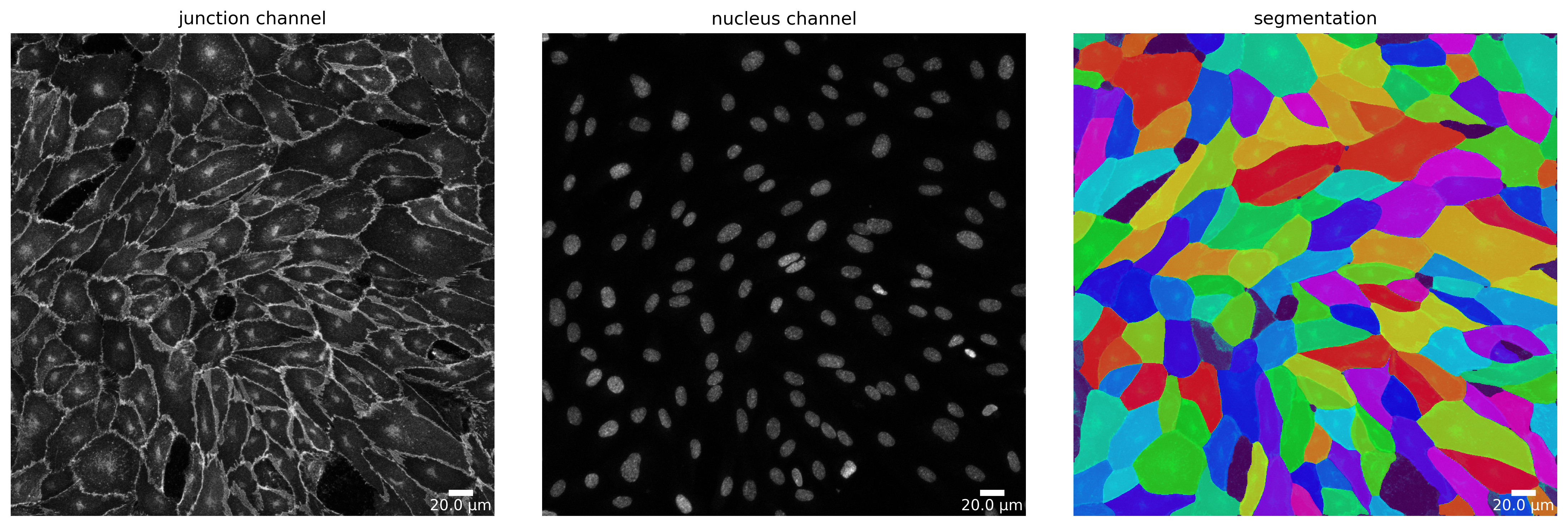
mask = cellpose_segmentation.segment(img_prepared, input_file)
# plot segmentation mask to check the quality
plotter = Plotter(params_plot)
plotter.plot_mask(mask, img_prepared, img_prepared_params, output_path, output_file_prefix);
[15]:
# feature extraction
collection = PropertiesCollection()
extractor = Extractor(params_runtime)
extractor.extract(img, params_image, mask, output_file_prefix, output_path, collection);
[16]:
collection.dataset.head()
[16]:
| filename | img_hash | label | cell_X | cell_Y | cell_shape_orientation_rad | cell_shape_orientation_deg | cell_major_axis_length | cell_minor_axis_length | cell_eccentricity | ... | junction_perimeter | junction_protein_area | junction_mean_expression | junction_protein_intensity | junction_interface_linearity_index | junction_interface_occupancy | junction_intensity_per_interface_area | junction_cluster_density | junction_cue_directional_intensity_ratio | junction_cue_axial_intensity_ratio | |
|---|---|---|---|---|---|---|---|---|---|---|---|---|---|---|---|---|---|---|---|---|---|
| 1 | 060721_EGM2_18dyn_02 | 99b1548d1d7368b24afd215aa00c0506a0f31434 | 11.0 | 721.049684 | 44.831045 | 3.115089 | 178.481461 | 148.218110 | 57.849774 | 0.920687 | ... | 356.551299 | 2243.0 | 317.373711 | 995720.0 | 1.050856 | 0.578093 | 256.628866 | 443.923317 | 0.076623 | 0.516027 |
| 2 | 060721_EGM2_18dyn_02 | 99b1548d1d7368b24afd215aa00c0506a0f31434 | 12.0 | 57.170727 | 55.504237 | 0.007508 | 0.430191 | 99.033516 | 76.261338 | 0.637976 | ... | 315.563492 | 1793.0 | 242.299719 | 619673.0 | 1.085897 | 0.559788 | 193.466438 | 345.606804 | -0.282458 | 0.587275 |
| 3 | 060721_EGM2_18dyn_02 | 99b1548d1d7368b24afd215aa00c0506a0f31434 | 13.0 | 619.520117 | 70.120408 | 2.742737 | 157.147232 | 102.321920 | 89.083348 | 0.491959 | ... | 334.534055 | 2079.0 | 267.149868 | 736250.0 | 1.070077 | 0.610932 | 216.353218 | 354.136604 | -0.131366 | 0.428645 |
| 4 | 060721_EGM2_18dyn_02 | 99b1548d1d7368b24afd215aa00c0506a0f31434 | 14.0 | 176.148852 | 105.566653 | 0.422114 | 24.185359 | 187.633346 | 145.493784 | 0.631451 | ... | 609.126984 | 2496.0 | 227.167310 | 1017159.0 | 1.065744 | 0.401544 | 163.635618 | 407.515625 | -0.262354 | 0.540647 |
| 5 | 060721_EGM2_18dyn_02 | 99b1548d1d7368b24afd215aa00c0506a0f31434 | 15.0 | 822.559345 | 71.767302 | 2.477095 | 141.927109 | 75.120572 | 52.348251 | 0.717211 | ... | 224.651804 | 1793.0 | 389.570198 | 816943.0 | 1.055555 | 0.772179 | 351.827304 | 455.629113 | -0.024172 | 0.541412 |
5 rows × 66 columns
[17]:
collection.dataset.to_csv(output_path.joinpath('features.csv'))
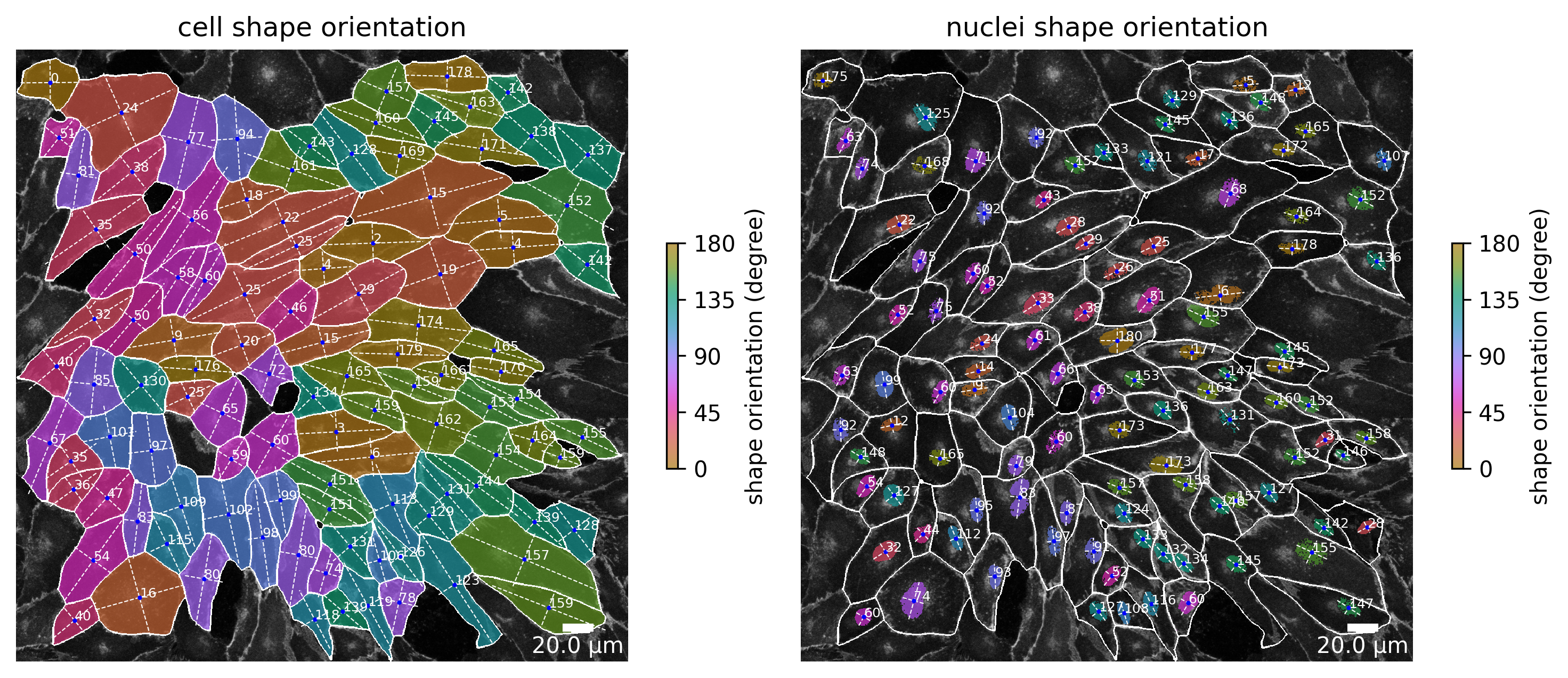
[18]:
# plot the cell orientation
plotter.plot_shape_orientation(collection, "060721_EGM2_18dyn_02");  # image is automatically saved in output_path